Installation Instructions and User Guide for ArcGIS Pro

Overview

Goal: Use the Rate Stabilizer Tool (RST) to produce easily mapped age-standardized, smoothed sub-county estimates.

Objectives: Gain experience installing the tool and managing the user interface. Develop an understanding of the required data inputs. Interpret and map the output.

Problem: You have been provided with individual level heart disease death data for the years 2006 to 2008 that have been geocoded to the U.S. 2010 Census tract level. Using the Rate Stabilizer Tool (RST), you will generate age-standardized, smoothed rates. Using the information generated by the RST, you will be able to map tract level death rates for heart disease for the state of North Carolina.

*** Files needed for exercise: NC_HeartDisease0608.dbf, and North Carolina census tract shapefile: NC_tracts_2010prj.shp

Obtain a U.S. Census API key

Go to Census Key Sign up site; fill all blanks: https://api.census.gov/data/key_signup.html

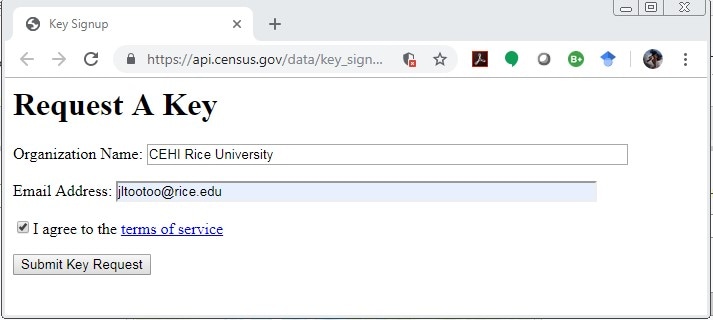
In a few minutes you should receive an e-mail like this:

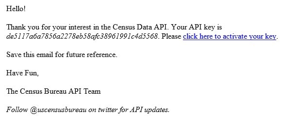
Activate your key and you are ready to use the Census API. You will need to use this key after you have downloaded the RST toolbox.

Loading the toolbox

1. Download the tool.
a. Save the zipped file to your workspace folder
b. Extract zipped file to your workspace folder

This tool has been built using Python and can be added as a toolbox into the ArcGIS Desktop interface.

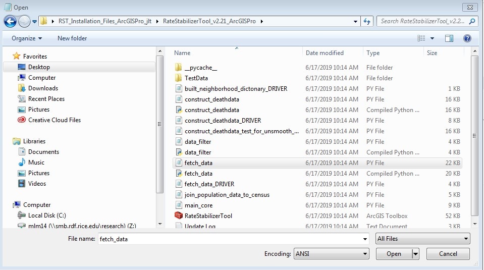
2. Add your API key. In your workspace folder RST folder, use notepad to open fetch_data.py

In line 14, paste the API key that you received from the U.S. Census email.

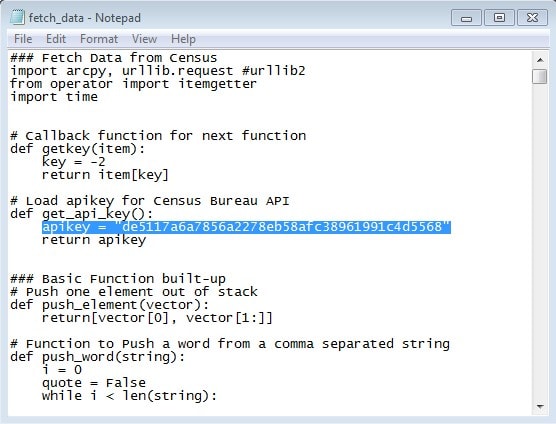
Close the fetch_data.py and save your changes.

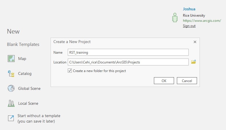
3. Go to ArcGIS Pro. Create a new map project in ArcGIS Pro.

4. Activate the Catalog pane by left clicking on the View tab on the top ribbon and click on Catalog Pane.

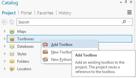
5. Right click on the Toolboxes icon at the top of the Catalog and select Add toolbox.

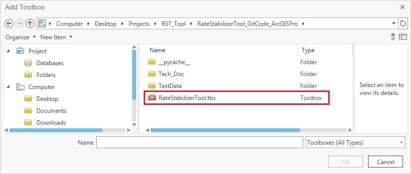
6. Navigate to your workspace location (where you extracted the toolbox). RateStabilizerTool_v2.20_ArcGISPro> RateStabilizerTool.tbx and click OK.

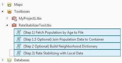
7. The RateStabilizerTool toolbox will now appear; expand the toolbox to reveal all of the script-based tools in this toolbox.

Adding your data

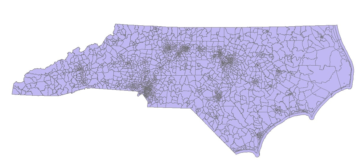
1. Select Add Data in the Map Ribbon. The 20_ArcGISPro TestData folder contains a shapefile: NC_tracts_2010prj.shp. Add this shapefile for some geographical context.

2. Next add the record level heart disease death data: NC_HeartDisease0608.dbf

Right click on the table name to view this table and take a look at the attribute fields:

• OID: an automatically generated object identifier.
• OBJECTID: automatically generated unique identifier.
• GEOID10: the geographic identifier for the U.S. Census tract unit that you will be calculating a stabilized age-standardized rate; this is a required field for the tool.
• DDR_ID: the unique-identifier for each record.
• Yr_Death: the year of the death record.
• Age: the age at which the individual represented by the record died; this is also a required field for the tool.
• Male: the sex of the decedent, with 1 indicating male and 0 indicating female (to be used in a future version of the tool).
• GEOIDCNTY: alternatively, the geographic identifier for the U.S. Census county unit can also be used to calculate a stabilized age-standardized rate.

Using the tool

This tool makes use of the U.S. Decennial Census API to obtain census population data for age-adjustment calculation.

First run the Fetch Population Age to File tool in the open environment to download the latest U.S. Census data from the U.S. Decennial Census API. Next, run the Rate Stabilizing Tool with Local Data tool in a secure environment – pointing to the U.S. Census data saved data in a secure location (behind a firewall for example).

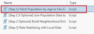
1. First run the (Step 1) Fetch Population by Age to File Script tool. Double left click on the icon to open the tool.

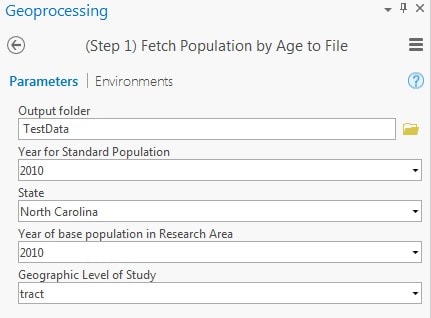
2. Let’s consider each of the parameters/inputs.

• Output folder: The output folder location for the results. Select your workspace folder as the output folder and then click “Ok” on the lower right side of the dialog box.
• Year for Standard Population: To standardize for age, you need to select a standard population. A standardized rate weight will be generated from the standard population. Select 2010 as the desired year of the standard age structure for the entire US.
• State: Select North Carolina as the state for which population data will be used to generate crude rates.
• Year of base population in Research Area: Select 2010 since our data was collected from 2006 – 2008. 2010 is the year of the chosen state’s base population that will be used for calculating crude rates.
• Geographic Level of Study: Select U.S. Census Tract as the desired geographic level of analysis for the population data.

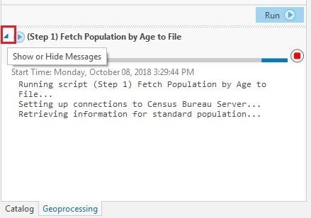
Click Run to run the tool… and expand to show messages. You should see this:

Once the tool has successfully run (the dialogue box will say “completed script” and “succeeded”). It will generate a data file that can be used to run the tool behind your firewall. In our case, the file will be named: RawData_state37_tract.data. This file can be re-used for multiple analyses.

3. The RST tool can optionally perform spatial Bayesian smoothing when given a neighborhood dictionary. Run the (Step 2 Optional) Build Neighborhood Dictionary Script tool to generate a matrix of adjacency relationships between geographic units. Double left click on the icon to open the tool.

4. Let’s consider each of the parameters/inputs for the tool.

• Shapefile for Spatial Bayesian: Select a shapefile containing all the geographic units at the level of study for the state of interest. The neighborhood dictionary will be built based on this input shapefile – select: NC_tract_2010prj.shp shapefile.
• GeoID in shapefile: Index the field name containing each geographic unit’s GeoID. In order to generate a valid neighborhood dictionary, you need a field containing a unique identifier for each census geography that aligns with the census ID; select– GEOID10.
• Output folder: The output folder location for the results. Single click your workspace folder and then click “Add” on the lower right side of the dialog box.

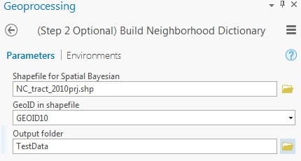
Click Run to run the tool. You should see something like this:

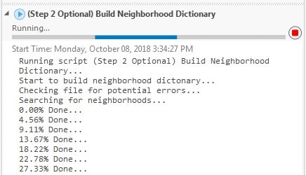
After the tool has successfully run, it will generate a new neighborhood_dict.data file. In our case, the file will be named: NC_tract_2010prj_neighborhood_dict.data.

5. Now that we have the population data from the U.S. Census to manage a proper age adjustment tool locally, and a neighborhood dictionary for optional spatial smoothing, we can run the (Step 3) Rate Stabilizing with Local Data Script tool. Double left click on the icon to open the tool.

6. Let’s consider each of these parameters/inputs for the tool.

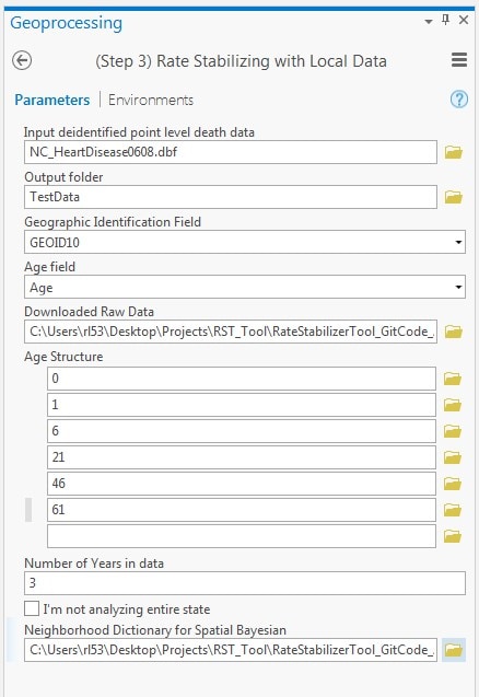
• Input de-identified point level death data: Select your records table for calculation. The age and GEOID fields are required for the calculation. Please de-identify the point level data before using the tool. Browse to the NC_HeartDisease0608.dbf file.
• Output folder: Select the output folder location for the results. Please single click your desired folder and then click “Add” on the lower right side of the dialog box.
• Geographic Identification Field: Index the field name containing the GeoID.
• Age field: Index the field name of the patient’s age.
• Downloaded Raw Data: Point the tool to the folder that you have placed the downloaded Census data (data). Remember in generating this data you have:
  • Selected Year for standard U.S. population 2010. In order to adjust for age, a standard population must be selected. The adjusted weight will be generated from standard population.
  • Selected the State of interest: NC or 37.
  • Selected the Year of base population 2010 for NC.
  • Specified the geographic level of study: Tract.

• Age Structure: Specify your own age group structure. Enter the lower-bound of each age group. One negative value can be used to control the max age of consideration. For example, for the following group structure:
  • Younger than 1 years
  • 1–5 years
  • 6–20 years
  • 21–45 years
  • 46–60 years
  • over 61 years

• The following numbers should be entered: 0, 1, 6, 21, 46, 61 (pressing enter to add the next value). For an age group structure:
  • Younger than 5 years
  • 5–10 years
  • 10–17 years

• The following numbers should be entered: 0, 5, 10, -18.
• Number of Years in data: Enter the total number of years represented by the input death data. Decimals can be used to represent partial years. For our example, enter 3.
• I’m not analyzing the entire state: Check this if your input data only reflects a portion of the state’s geographies rather than the entire state. Why? If we tell the tool that the base population is for the entire state, it will smooth to that population. If the data only comes from select counties, we only want to consider the base population for these counties combined. For our example, uncheck this box since we are analyzing data from every county in North Carolina.
• Neighborhood Dictionary for Spatial Bayesian (optional): If you would like to include spatial Bayesian smoothing, select the neighborhood dictionary data file built in Step 2. Otherwise, leave blank. Navigate to and select the NC_tract_2010prj_neighborhood_dict.data file and select “Open”.

Here is what your completed test run of the tool should look like once you have input the parameters:

Let’s talk about what is going on while the script is running:

• The tool is using the census data file you created to calculate population in each age group and the standard age structure.
• The tool is calculating crude rates for each age category you specified. Once these are calculated, age-standardized rates (both smoothed and non-smoothed) are calculated for each age category and standard age structure.
• If there are GeoIDs (census Identifiers in this case) that are missing, or cannot be recognized in census data, you will receive a warning.
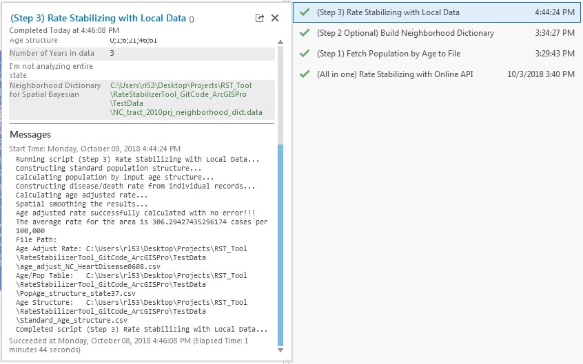
• All output file paths can be viewed under the Messages section in the Analysis > History Pane.

Understanding the output

1. Once the tool has completed all processes, three tables will be placed in the Output folder you specified. These include two intermediate tables required for calculations which can be used for verification:

• PopAge_structure_state37.csv: This file includes the population for each geographic unit in the state of interest by age category. You defined these age categories when you set up the tool.
• Standard_Age_structure.csv: This file includes the proportion of the population in each age category in the standard year of choice. This age structure was calculated using the population data from the whole United States. The structure works as the weight when calculating the weighted average for age-standardized mortality rate.
• And the table with your results: age_adjust_NC_HeartDisease0608.csv

2. Add the results table to ArcMap and open it up to see what has been produced.

• Age_adjust_rate: the non-smoothed rate per 100,000
• SpBay_AAR: the spatially smoothed rate per 100,000
• SpBay_2p5 & SpBay_97p5: the lower and upper boundaries for 95% confidence interval for spatially smoothed age-standardized rate
• Baye_AAR: the smoothed rate per 100,000
• Baye_2p5 & Baye_97p5: the lower and upper boundaries for 95% confidence interval for smoothed age-standardized rate.

3. Potential Alert Messages: When the width of the confidence interval (Upper limit – Lower limit) is larger than the estimate, the estimate is unreliable. These rates should NOT be mapped.

• Alert: Unreliable Empirical Bayesian Estimate!!! – The empirical Bayesian estimate is not reliable in the region.
• Alert: Unreliable Spatial Bayesian Estimate!!! – The spatial Bayesian estimate is not reliable in the region.
• Alert: Unreliable Estimate!!! – Both estimates are not reliable in the region.

4. NSpUnreli: New after version 2.15. This field indicates the reliability of non-spatial Bayesian estimates. Non-spatial Bayesian will be reliable if NspUnrel is 0.

5. SpUnreli: New after version 2.15. This field indicates the reliability of spatial Bayesian estimates. Spatial Bayesian will be reliable if SpUnrel is 0.