At a glance
Introduction to R0 and Rt
The basic reproductive number, R0 (pronounced R-naught), is defined as the expected number of new infections caused by each infected person in a fully susceptible population in the absence of interventions (e.g., vaccination, social distancing, or masking). R0 is an important theoretical concept in epidemiology, but in the real world, a fully susceptible population rarely exists.
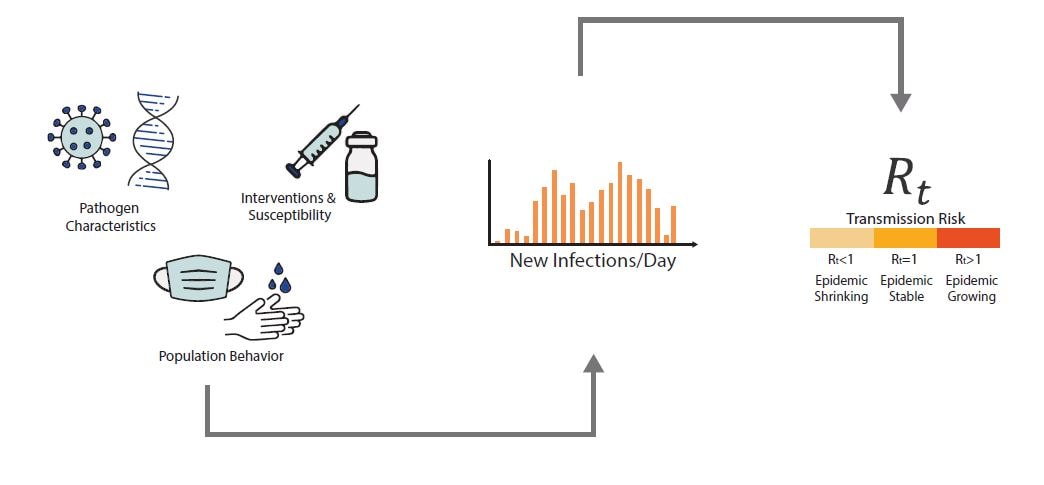
The time-varying reproductive number, known as Rt, is defined as the average number of new infections caused by each currently infectious person at time t—reflecting current population susceptibility, behavior, public health interventions, and variant transmissibility at the time it is measured (Fig. 1). It is a data-driven metric of transmission, unlike R0.
When Rt is above one, infections are increasing because, on average, each infected person is causing more than one new infection; when Rt is below one, infections are decreasing. Rt can provide early indication of increases or decreases in cases, hospitalizations, or deaths, because transmission occurs before case confirmation, hospitalization, or death.
An epidemic's growth and decline are driven by underlying changes in transmission over time. Early in an epidemic of a novel disease, when no one has prior immunity, transmission rates are usually highest. Rates then decline as people change their behavior to avoid infection, or gain immunity through infection or immunization. The peak of an epidemic is a turning point that occurs when transmission falls below a critical threshold where, on average, each infected person no longer causes more than one new infection.
Rt cannot be measured directly, instead, Rt is estimated from data. During an epidemic, Rt estimates provide information about the trend of the epidemic and can be used to forecast short-term changes in cases, hospitalizations, or deaths, and to assess the effectiveness of interventions designed to slow transmission. Other trend metrics may measure changes in emergency department visits, hospitalizations, or deaths, which are delayed outcomes of new infections.
Rt alone cannot tell us why an increase or decrease might be occurring. Changes in behavior, vaccination coverage, levels of immunity from infection, other factors, or a combination of these factors can affect Rt. Additional data are required to assess reasons for the trends summarized by Rt.
Key takeaways for public health
Rt is a transmission metric that estimates the ratio of infected people to infectors in an epidemic at a particular point in time. Rt estimates help inform situational awareness, giving clues as to how quickly an epidemic is likely to increase or decrease in the near future. To be useful for decision making, Rt estimates need to be accurate, accounting for time lags because transmission events causing cases now occurred days to weeks ago.
Rt allows public health decision-makers to assess the impact of interventions because it estimates how transmission rates have changed over time, and to assess the intensity of spread because it directly reflects growth in infections.
A real-world application of Rt is CDC's Epidemic Trends for seasonal respiratory diseases. In 2024, CFA collaborated with the New Mexico Department of Health to assess the performance of CDC's epidemic trends and found that epidemic trends were an early indicator of increases in SARS-CoV-2 (the virus that causes COVID-19) community transmission, before detection in other surveillance data. Additionally, epidemic trends were a confirmatory indicator that decreases in the number of ED visits for COVID-19 were due to true decreases in transmission, rather than delayed reporting.
Measuring transmission with Rt
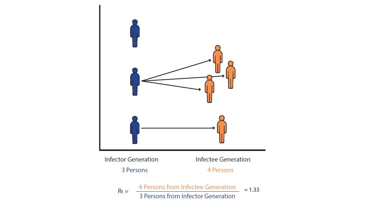
Let's imagine a world in which we can observe every disease transmission event exactly when it occurs. In this hypothetical world, we count the number of new infections that occurred on day t and divide by the number of infected persons who caused them, to give us Rt: the average number of new infections that each previously infected person caused (Fig. 2).
In reality, it's almost impossible to know exactly when transmission occurred or who infected whom in epidemiological data. While sometimes epidemiologists run focused studies designed to observe transmission events and transmission chains, these studies require intensive monitoring of a small group of participants and are the exception, not the rule. To get around these challenges, we estimate Rt using data that are relatively easy to obtain: daily counts of the number of new cases, emergency department visits, hospitalizations, or deaths. We input these data into a mathematical model designed to deal with three main challenges of data observation:
To estimate Rt, we need to divide the total number of newly infected people on day t by the number of people who caused those infections (Fig. 2). But how can we do this if the data only contain counts of the total numbers of infections observed each day?
Note
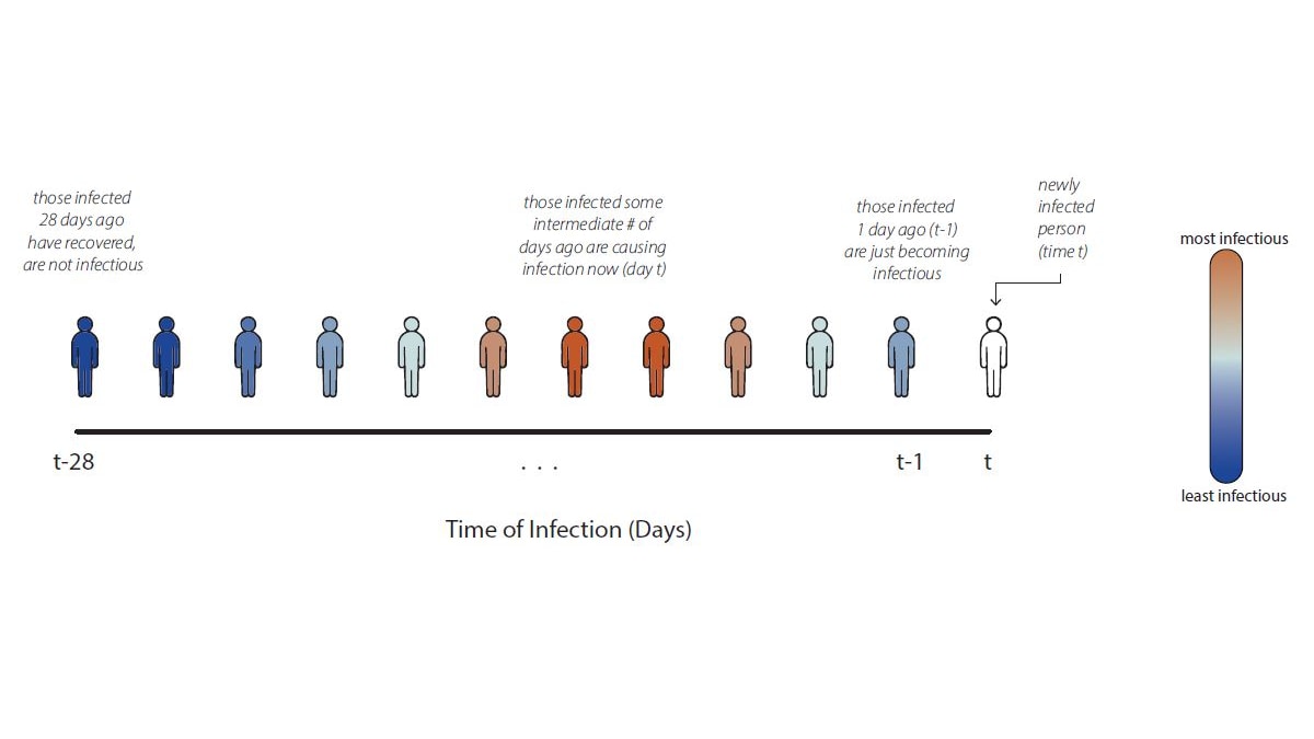
In count data, we can directly read the numerator of the Rt ratio—the number of newly infected people on day t—from the data. The denominator is more difficult to assess. Instead of trying to infer exactly who infected whom, we make assumptions grounded in infectious disease biology. For SARS-CoV-2, for example, we know that individuals infected yesterday need time to become infectious as their viral loads increase. Meanwhile, individuals infected weeks ago have likely recovered and are no longer infectiousA. We can assume that individuals who were infected some intermediate number of days in the past are now causing the bulk of new infections (Fig. 3).
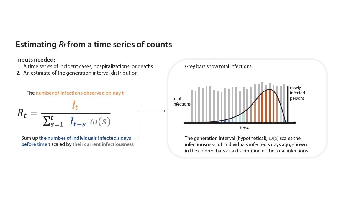
To estimate Rt, we must develop a model that turns the assumption "individuals infected some days in the past are the ones causing transmission now" into an equation. Our equation is a more complex version of the Rt ratio in Fig. 2, inferred using observable variables. To count the number of individuals in the infector generation on day t, we need to sum across all the individuals who became infected in the recent past—starting yesterday and going back weeks ago—weighted by their current infectiousness (Fig 4). For SARS-CoV-2, we assume that individuals infected between 1 and 7 days ago are most infectiousA, but individuals infected earlier or later may still cause infections. Different assumptions about the generation interval, or time between a person becoming infected and passing that infection to someone else, can result in different estimates of Rt.
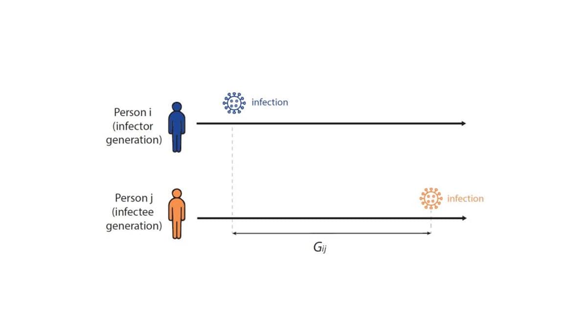
To formally estimate how long the expected wait between infections in a chain of transmission is—and to establish the infectiousness weighting function in Fig. 4 above—infectious disease models use a distribution called the generation interval (G), defined as the interval between the infection times of an infector-infectee pair (Fig 5). For example, if person i was infected on Monday, and if person i infects person j on Friday, then the Gij is four days. We know that the generation interval varies between transmission pairs, and so we want the distribution of times between infector-infectee pairs. We can estimate the generation interval distribution using data from household or contact tracing studies, in which the approximate timing of infections is observed, or by using the serial interval (the time between onset of symptoms of an infector-infectee pair) as a proxy.
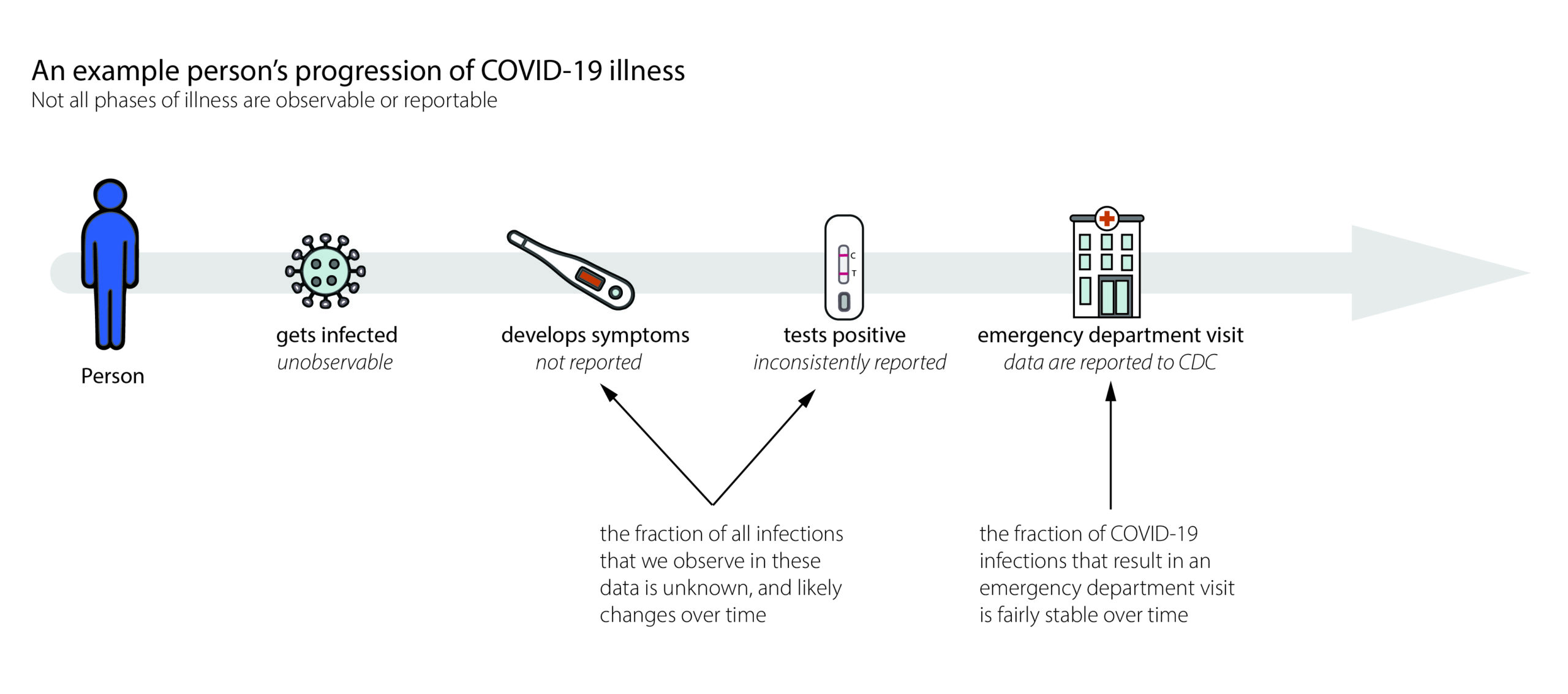
When we estimate Rt, we want to know how many new infections occur on day t. In the real world, we observe events like cases, emergency department visits, hospitalizations, or deaths with delays of days to weeks (Fig. 6). These delays are unavoidable and fall into two main categories:
- Biological delays between the moment a person is first infected and the moment their infection could become observable and/or reportable as a confirmed case, emergency department visit, hospitalization, or death, and
- Reporting delays between the time a person tests positive, visits an emergency department, is admitted to the hospital, or dies and the time that event is reported to the health department. Data from some events, like positive at-home tests, may never be reported and are therefore difficult to reliably or completely count (Fig. 6).
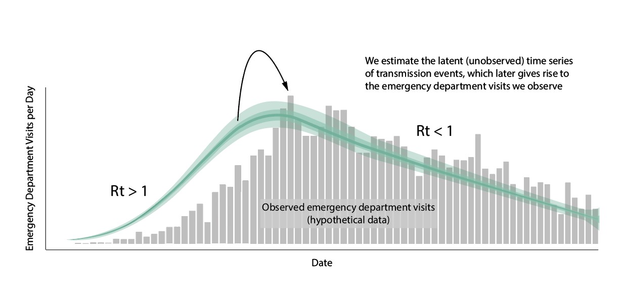
As a result of these delays, it is possible that Rt estimates sometimes show an increasing trend while trends in observable outcomes are showing declines. This is because Rt estimates focus on estimated trends in infections; we expect to see infections increase before observable events, such as numbers of ED visits, given the natural delay between a person's infection and severe outcomes, like an ED visit or a hospitalization (Figure 7).
Caveats and complications:
- On the most recent dates, we have not yet observed all infections that will be reported, as some infected people have not yet developed symptoms or visited an emergency department. This is a challenge because people are usually most interested in recent trends, but recent data are incomplete.
- There are day-of-week effects in healthcare visits and reporting, where the data consistently show more reports on weekdays vs. weekends.
- Events (e.g., positive tests, emergency department visits, hospitalizations, deaths) are not always reported on the day that they occur. For example, sometimes test results take a few days to come back from the lab, diagnoses undergo review, or there are delays in transferring data.
To adjust for incomplete reporting on recent dates, CDC implements "nowcasting" approaches to predict the final observed counts that will eventually be reported, based on incomplete preliminary counts available today and reporting delays measured from recent data.
In any data, we only observe a fraction of infected individuals—those that were detected and reported as testing positive, or visited the emergency department and were diagnosed with that infection, or were hospitalized (Fig. 8).
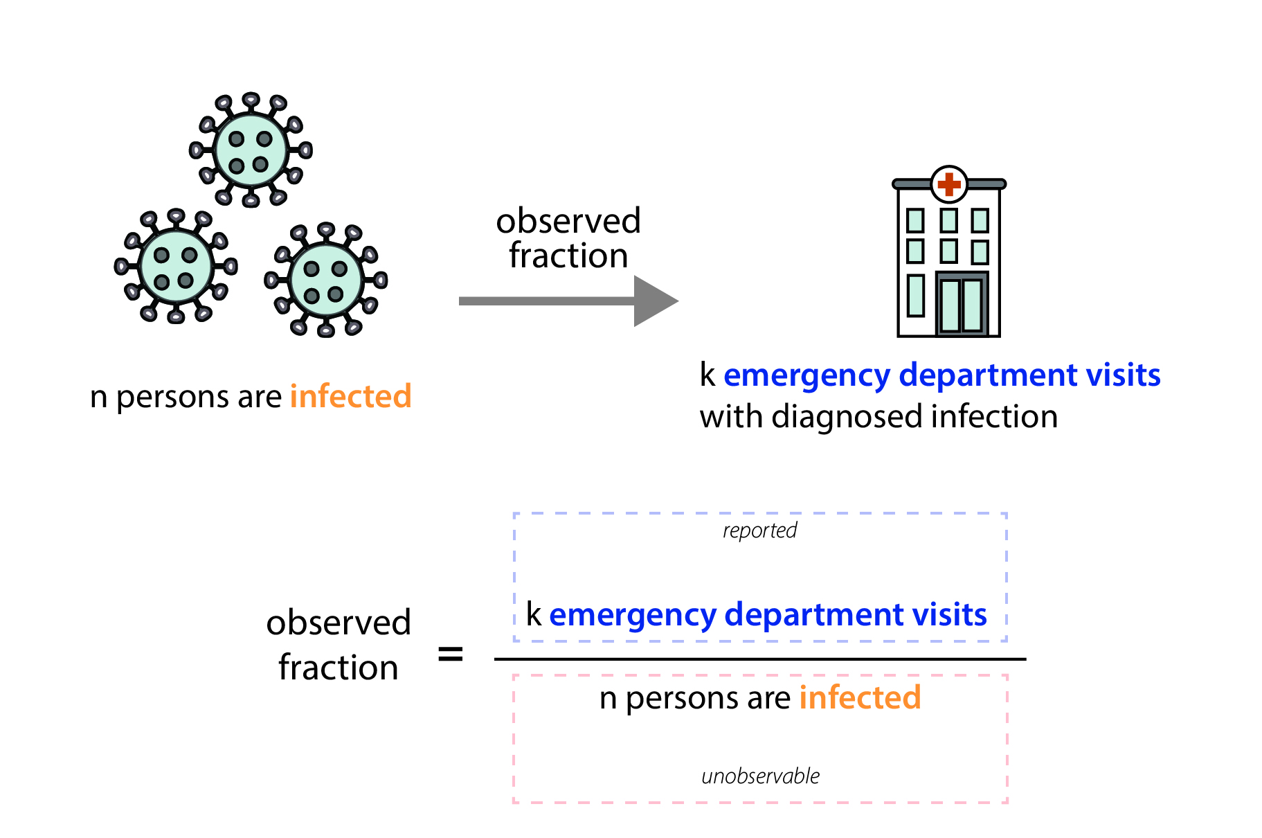
Mathematically, we expect our Rt estimates to be unbiased as long as the fraction of observed infections is not changing rapidly. That is because the observed fraction impacts both the numerator (the infectee generation) and denominator (the infector generation) of our Rt equation equivalently (Fig. 9). In reality, there is probably no epidemic dataset where there is no change at all in the fraction of observed infections over time. Additionally, there are some situations where the fraction of observed infections could change quickly enough to temporarily cause over- or under-estimates of Rt, such as the emergence of a more severe variant, lack of diagnostic tests, a clinical or testing practice change within a healthcare setting, or changes in reporting.
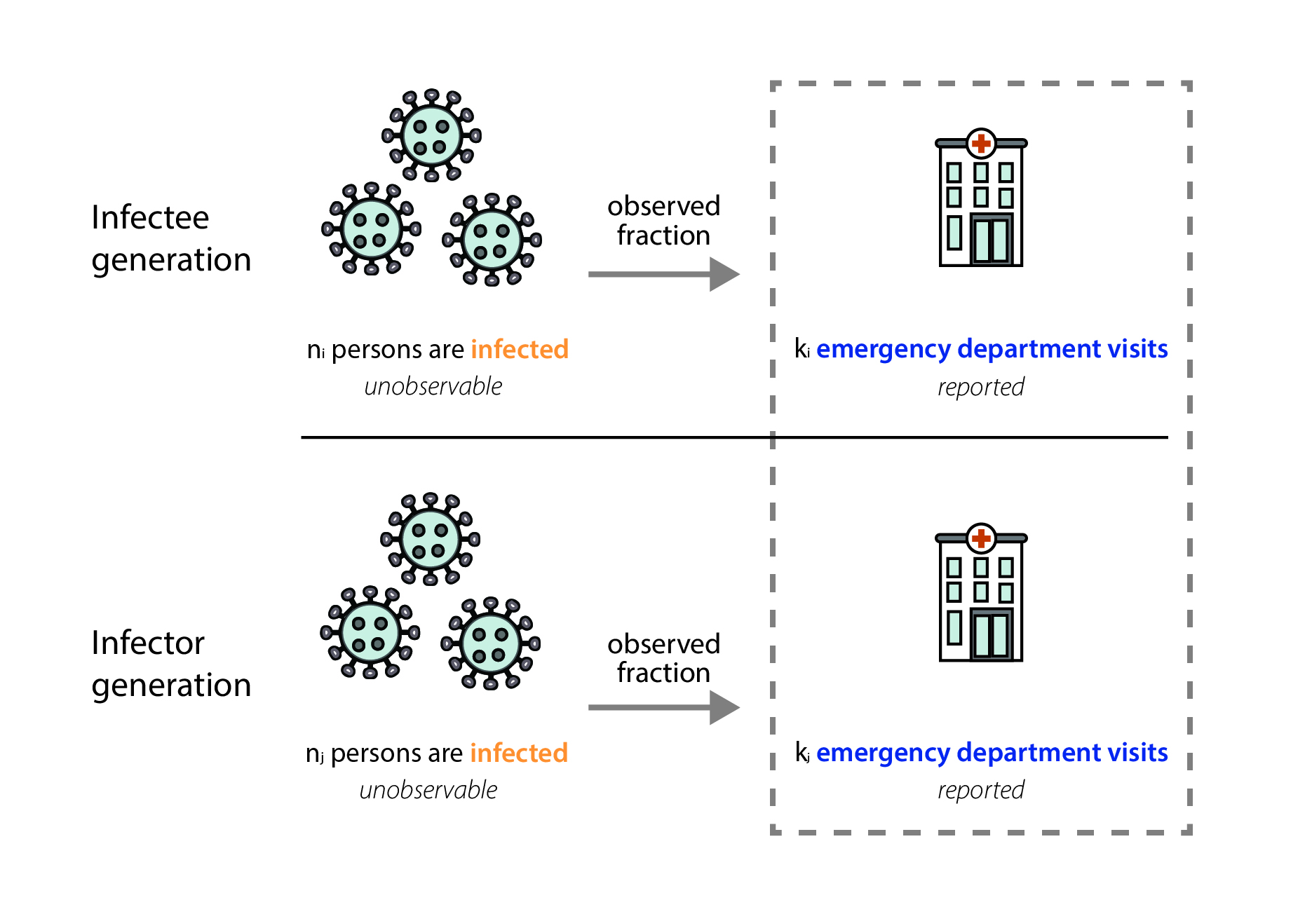
It is important to note that whichever data source you choose, those individuals could be systematically different from the general population. For example, individuals visiting the emergency department for respiratory illness may be older, have other coexisting medical conditions, or limited access to other healthcare options (e.g., primary care or urgent care). However, these differences don't directly affect Rt estimates, because we are not measuring the number of new infections that specific individuals go on to cause. Instead, Rt estimates reflect the population average level of transmission that caused those individuals to become infected themselves.
In fact, though counterintuitive, in an epidemic system without rapid changes in severity, infectiousness, or precautionary behavior, different age groups should experience roughly similar epidemic growth rates over time after an initial mixing period. Although the total number of infections in each group will be different, the relative change should be the same. This means that estimates of Rtbased on incident events from a subgroup (individuals who visit the emergency department, for example) of a population are unbiased as long as the fraction of observed infections in that subgroup stays roughly constant.
Methods for estimating Rt
There is no single universal method to estimate Rt; several packages, or specialized programming toolkits, are available for estimating Rt in R. This decision matrix from partners at Boston University provides an overview of major considerations needed to decide on a method and its associated programming package(s). Briefly, one should consider the desired output (nowcasting, forecasting, or historical evaluation), whether and which delay distributions should be included, theories and assumptions made in the method, and level of documentation available for a new user to be able to apply the method on their own. Information about how CFA estimates Rt for seasonal respiratory viruses can be found in our Behind the Model on Assessing Epidemic Trends.
Learn More About How We Estimate Rt
See video featuring CDC scientist Katie Gostic on how to calculate Rt
Evaluating Rt estimates
In some epidemic modeling analyses, we get to check our answers. For example, if we generate a short-term epidemic forecast, we can wait a few weeks and then check our predictions against what really happened. But we're never able to observe Rt directly, and so we don't have a gold standard source of truth to check our models against. As a result, we use a few different methods to check that our estimates are reliable.
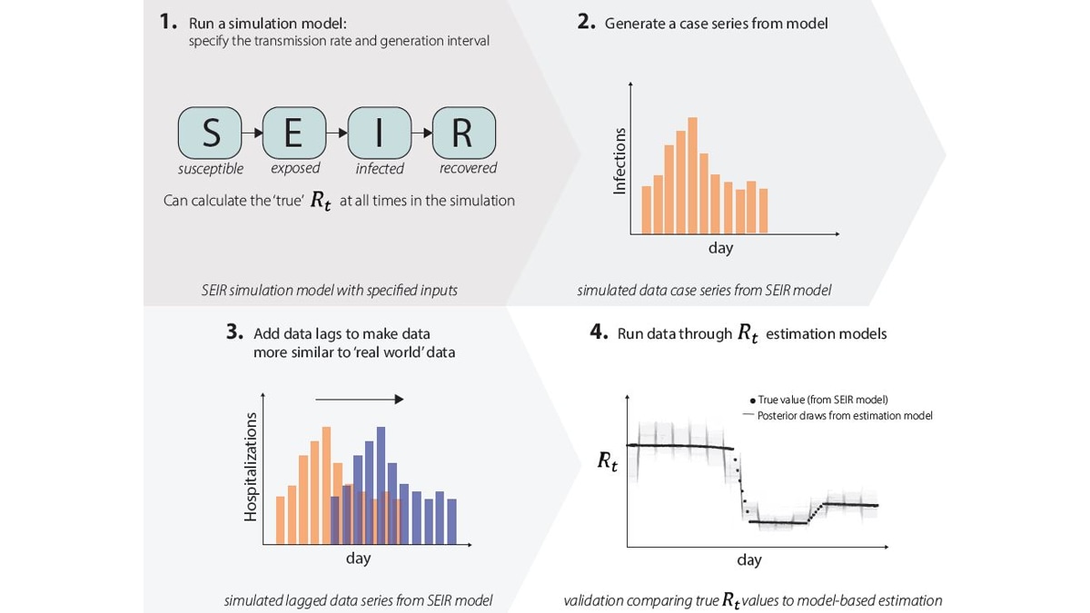
- We run simulation studies. We run an epidemic simulation using a dynamic mathematical model with four compartments: susceptible (S), exposed (E), infected (I), and recovered (R) (Fig. 10.1) where we can calculate the 'true' Rt value at all times. The simulation produces an epidemic time series with counts of the number of new infections per day (Fig. 10.2), and we add lags to these data to make them more similar to the case, hospitalization, or death data that we observe in the real world (Fig. 10.3). We can run these simulated data through our Rt estimation models just like real data, only in this case we know exactly what the answer (Rt) should be, as we specified it when simulating the data. We then compare results to the correct answers (Fig. 10.4). If our models do not accurately estimate Rt, we know we need to make changes until the model accurately estimates Rt.
- We check that our real-time estimates are consistent with observed trends. We compare estimates with each other to ensure they are reasonably consistent over time as new data become available.
- We perform common-sense checks. If the data show that the epidemic is growing rapidly, then we should see Rt estimates, including confidence intervals, above one for the corresponding time period, after adjusting for lags.
- We evaluate nowcasts and short-term forecasts from our models. We validate that the models consistently estimate final reports accurately, using the partial information available at the time.
Rt differs from short-term forecasting
Rt is one way to summarize the information generated by a short-term forecast. Rt estimates the trend in the number of infections in the coming days, 1) assuming current trends continue in the short-term, and 2) it does not tell us anything about level of disease activity. Short-term forecasting provides an estimate of expected disease activity over the coming weeks—both how high the activity is, and whether and how it is changing in the near future. For examples of short-term forecasts, visit our Behind the Model on Short-term Forecasts.
- Day 1-7 covers the central 95% of the generation interval distribution for Omicron from Park et al., 2023; day 1-5 covers the central 80% of the generation interval distribution. See Figure 5 for a definition of the generation interval.