Behind the Model: CDC's Tools to Assess Epidemic Trends

Current Epidemic Trends

CDC estimates epidemic trends, based on the time-varying reproductive number (R_t), for respiratory diseases at the national, state, and health service area (HSA) levels.

Epidemic trend estimates indicate whether infections are increasing (R_t > 1) or decreasing (R_t < 1). Read more about how to interpret R_t estimates in our Modeling Handbook chapter on R_t and see how the real-world application of R_t helped detect an early increase in COVID-19 activity in this MMWR article.

R_t is estimated from data because it cannot be measured directly

R_t is a measure of community disease transmission and is defined as the average number of new infections caused by each currently infectious person at time t. R_t is an unobservable value that, as the name implies, varies over time depending on dynamic factors such as pathogen characteristics, population susceptibility and behaviors, and current public health interventions. Because transmission is difficult to directly measure, R_t must be estimated from observable epidemic data such as positive tests, emergency department visits, hospital admissions, or deaths caused by a specific disease. Transmission varies over the course of an epidemic, so informative and timely R_t estimates should be updated at regular intervals.

Below is a walk-through of the basic logic, assumptions, strengths, and limitations of the model and data CFA uses to estimate R_t; those with technical backgrounds may also wish to review more details of our approach. For a more introductory background on the concept of R_t and how it is useful in public health decision making, please read our Modeling Handbook chapter on R_t.

The Data: Syndromic surveillance emergency department visits

CDC estimates R_t from emergency department (ED) visit data reported through the National Syndromic Surveillance Program (NSSP). ED visits serve as a proxy to estimate current transmission trends under the assumption that they represent a consistent fraction of new infections over time. We use ED visits because they provide one of the most stable fractions of infections of any available data source (Evaluating Data Types, 2020), unlike positive tests or symptomatic case reports, which can be highly variable over time. The exception to this stability is when there is a shift in disease severity—such as may be caused by a new variant—or a rapid change in access to care or care-seeking behavior. If such a situation occurs, we will add a note to our webpage that there is some possibility of inaccuracy during the brief period before the fraction observed re-stabilizes.

A second advantage of using ED visits as a proxy for transmission is timeliness. ED visits occur soon after the initial infection and are reported quickly to NSSP. Other signals can be stable, but much more lagged. For example, disease-related deaths may not be reported until weeks or months after the initial infection (Evaluating Data Types, 2020).

Reporting ED visits to NSSP is voluntary, but there is widespread coverage across the United States, and many participating facilities have automated reporting systems. At the state level, total reported visit volumes to NSSP are usually very stable over time. CDC monitors total reported visit volumes to ensure that reported R_t values reflect actual increases or decreases in transmission, not just increases or decreases in the amount of overall reporting from EDs. First, we run automated scans to detect anomalies in total reported ED visits from each jurisdiction. If these scans detect a potential issue with the data—that data may be missing, that a facility has temporarily stopped reporting visits, or that a facility has recently been added to the system—we can clean the data. Data cleaning may include dropping one or two unusually low or high reported values, filtering which facilities are included in R_t estimation, or—in the case of a more widespread reporting outage—choosing not to report an estimate for the affected jurisdiction until the problem is resolved. Second, to account for small daily fluctuations in reporting, we use an R_t estimation method that adjusts for changes over time in total reported ED visits.

The Output: Current epidemic trends at the state and local levels

As of June 2026, CFA—in collaboration with the National Center for Immunization and Respiratory Diseases (NCIRD) and the Office of Public Health Data, Surveillance, and Technology (OPHDST)—publishes weekly estimates of epidemic trends at the Health Service Area (HSA) level, in addition to the state and national levels. An HSA is a geographic area that combines one or more counties that are next to each other to form a region that is relatively self-contained with respect to hospital care. CFA uses NCI modified HSAs, where all counties within an HSA are in the same state. Jurisdictions that do not participate in data-sharing at this geographic scale for trend reporting are labeled as “data unavailable.”

Epidemic trend categories are determined by estimating the distribution of possible R_t values based on the observed ED visit data and model assumptions. We calculate the proportion of that distribution where R_t > 1. When R_t > 1, infections are increasing, so in simple terms you can think of epidemic trend categories as the probability that infections are increasing:

• If >90% of the distribution of R_t >1, infections are determined to be "growing";
• If 75%-90% of the distribution of R_t > 1, infections are "likely growing";
• If 25%-75% of the distribution of R_t > 1, infections are "not changing" (in this case, the distribution spans across 1, and contains a mix of values above and below 1.);
• If 10%-25% of the distribution of R_t > 1, infections are "likely declining"; this is equivalent to 75%-90% of the distribution of R_t ≤ 1;
• If <10% of the distribution of R_t > 1, infections are "declining"; this is equivalent to >90% of the distribution of R_t ≤ 1.

We do not estimate R_t in the following cases:

1. There is insufficient disease circulation to calculate a trend (specifically, there were no reported ED visits for the condition of interest on >20% of the dates in the past 8 weeks),
2. Recent sustained anomalies are detected in the number of reported ED visits (e.g., due to temporary data feed disruption), and/or
3. CFA's model does not pass checks for reliability—including checks for model convergence and manual review of estimates that are unusually high or low, potentially unstable, or have unusually large uncertainty.

The Model: A partially pooled, hierarchical generalized additive model for estimating R_t

The generalized additive model: As of June 2026, CFA uses a generalized additive model (GAM) to estimate R_t. A GAM is a generalization of linear regression—a type of statistical model, capable of estimating smooth relationships between predictors and the outcome. GAMs have previously been used by public health agencies for infectious disease nowcasting, forecasting, and R_t estimation.

To estimate the trend in infections (R_t) from observed and reported ED visits, the model first generates a nowcast and a short-term forecast of projected ED visits. The nowcast corrects recent partially reported data, based on historical reporting patterns, to estimate how many ED visits will eventually be reported. A short-term forecast then projects the expected number of ED visits in the next two weeks. Understanding that infections and ED visits are correlated—some fraction of today's infections will go on to visit the ED in the near future—the model then shifts backward in time to approximate the number of current infections. The direction (increasing, decreasing, not changing) between the estimated current number of infections and estimated future number of infections is the epidemic trend. The R_t estimate reflects the magnitude of the expected transmission per infected individual.

CFA's GAM estimates a smooth mean epidemic trajectory over time. The assumption of smoothness has the effect of stabilizing estimates, so that small changes in ED visit counts do not result in large swings in R_t estimates.

For more technical details about CFA's modeling methods, see 'Under the Hood' below.

Hierarchy

In our model, the R_t estimates for larger geographic units (e.g., states) are derived from the estimates of smaller units nested within it. Our model estimates R_t for all the smaller geographic units together.

One benefit of this hierarchical model structure is that sparse or missing data in one local-level jurisdiction does not negatively impact estimates at larger geographical scales. This approach improves accuracy and ensures estimates can still be reliably generated at higher levels, even during sporadic local data outages.

Another benefit is that this structure is highly flexible and can be applied to different geographic units. For example, right now, we display state-level and HSA-level trends. In the future, R_t estimates could be provided with any combination of counties, or even at finer levels of geographic resolution (Figure 1).

View Larger

Show More

Partial pooling

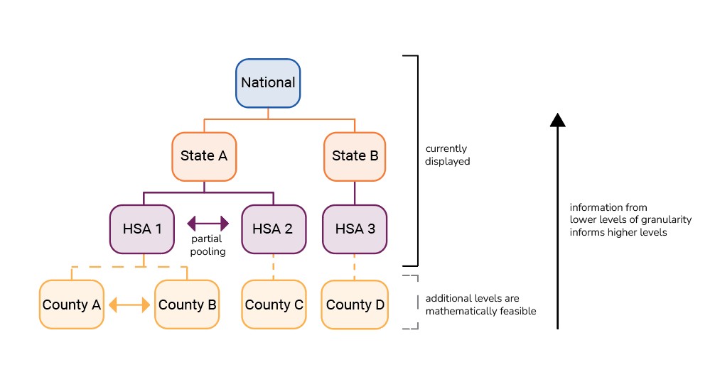
The model is also spatially partially pooled, meaning that each R_t estimate is informed by data from other elements within the same level of the hierarchy. For example, to generate a given HSA-level estimate, the model considers information from that HSA, all other HSAs within that state, and some nearby HSAs from neighboring states. Information is contributed proportionately; areas with more data, like larger HSAs, contribute more information to their respective pools. This approach helps to stabilize and inform estimates from areas with less data by bringing their estimate closer to the average R_t of the larger group.

Another benefit of the partial-pooling approach is that early trends identified in one area contribute that information to estimates for other areas, indicating potential upcoming disease activity in areas where it may not yet be detected. For example, increasing cases in a large metropolitan area (HSA 1) could indicate a possible upcoming increase in cases in a nearby smaller area (HSA 2); considering this information together, the model would adjust the R_t estimate for HSA 2 to be higher than if it were estimated without information from HSA 1. The model is geographically weighted such that neighboring elements—even across state lines —contribute information relative to their commute connectedness, determined from the most recent available version of commute flows from the US Census American Community Survey.

How do we evaluate CDC's R_t estimates?

We evaluate R_t similar to how we estimate it, by comparing our estimates to an observable proxy, namely ED visits.

We retrospectively compare the number of ED visits predicted by our model with the final observed ED visits from the NSSP surveillance data. We also compare the direction of the projected short-term forecasts from the GAM model to the actual percent change in the final reported ED visits. You can read more about evaluating short-term forecasts in our Behind the Model on short-term forecasts.

In 2024, we partnered with New Mexico Department of Health to show how our epidemic trend categories based on R_t (estimated by the previous EpiNow2 method) mitigated reporting lags in surveillance data to provide an early indicator of increases in COVID-19 community transmission and a confirmatory indicator that decreasing COVID-19 ED visits reflected actual decreases in COVID-19 community transmission.

Under the Hood: Technical details on CFA's methods

Adjusting for reporting effects to nowcast and forecast ED visits

Our R_t estimation methods rely on generating accurate nowcasts and forecasts, which require us to adjust for reporting effects. Our nowcasts and forecasts correct for three types of reporting effects: reporting delays, day-of-week effects, and overall ED visit volumes.

1. The reporting delay is the average amount of time between when someone is infected and when their case is reported. This delay is a key parameter for nowcasting. Correcting for the reporting delay allows us to estimate the current number of cases from incomplete or partially reported data.
2. Day-of-week effects account for differences in care-seeking behavior and case reporting that vary by day of week.
3. In order to separate changes in the disease of interest (the numerator) from changes in overall ED visit volumes (the denominator), the model is formulated as a rate regression using ED visits for all other conditions as an offset.

The model estimates all these effects together, for every county in the state of interest, and derives HSA-level estimates by combinations of the corresponding county-level estimates (Figure 2). To ensure continuity across state lines, the model is also trained on data from counties outside the state but in the state's commute network. Together, the estimated epidemic trajectory and corrections for reporting effects generate a nowcast and a short-term forecast of the number of ED visits occurring each day, in each jurisdiction.

View Larger

Show More

Estimating R_t from nowcasts and forecasts of ED visits

Once we have generated ED visit nowcasts, the estimated ED visits are transformed into an R_t estimate. Like the slope of a curve, R_t is a summary statistic that communicates whether we estimate that infections are increasing, declining, or not changing, based on the ED visit forecast. The same way that the slope of a line is defined by an equation, R_t is defined by the renewal equation (Figure 3), which contains two variables: the number of infections per day, I_t, and the generation interval distribution, ω(s). We estimate I_t from the ED visit forecasts and obtain a disease-specific estimate of ω(s) from the literature.

View Larger

Show More

Specifically, we approximate the number of ascertained infections per day by shifting estimated ED visits back in time by the mean delay from infection to ED visit, u, I_t = Y_t - u. (Subscripts for delay and jurisdiction have been dropped for clarity). The generation interval is the time between an individual becoming infected and them transmitting the infection to someone else. This parameter enables the model to estimate how infected cases already observed in the data are contributing to current community-level transmission.

How our current method compares to previous methods

From 2022 to 2026, CFA used a semi-mechanistic Bayesian model to estimate R_t at the state-level using the R package EpiNow2. This previous approach estimated R_t for each state independently and did not allow for efficient computational scaling to estimating R_t at the sub-state levels. Our current GAM method enables scaling to the greater number of sub-state estimates without requiring additional computational run time or compromising accuracy. Additionally, the hierarchical model provides more stable estimates in areas with low counts than the EpiNow2 approach.

We compared our R_t estimates from the GAM model to that of CDC's previous EpiNow2 R_t estimation method and found that R_t estimates from GAM matched or exceeded the one-week-ahead predictive performance of CDC's published EpiNow2 estimates in the 2024-2025 respiratory disease season.

Parameters we use to estimate R_t for COVID-19, influenza, and RSV

Disease-specific parameters
COVID-19
Generation interval distribution	Lognormal distribution with mean 2.9 days and standard deviation 1.64 days (Park et al. 2023), discretized with maximum 12 days and minimum 1 day.
Incubation period distribution	Modified Weibull distribution with mean 4.24 days (Park et al. 2023)
Distribution of delays from symptom onset to emergency department (ED) visit	Lognormal distribution with mean 4.17 days and standard deviation 6.27 days, discretized with maximum 30 days and minimum 0 days (from internal data)
Distribution of delays from infection to ED visit	Derived by combining the incubation period and delay from symptom onset to ED visit. Used to correct for the delay between infection and ED visit.
Influenza
Generation interval distribution	Gamma distribution with mean 3.52 days and standard deviation 2.10 days (Chan et al. 2024), discretized with maximum 9 days and minimum 1 day.
Incubation period distribution	Gamma distribution with mean 1.55 days and standard deviation 0.66 days (Chan et al. 2024), discretized with a maximum of 5 days, and a minimum of 0 days.
Distribution of delays from symptom onset to ED visit	Gamma distribution with mean of 3.52 days and standard deviation of 2.91 days, discretized with maximum 15 days and minimum 0 days (from internal data)
Distribution of delays from infection to ED visit	Derived by combining the incubation period and delay from symptom onset to ED visit. Used to correct for the delay between infection and ED visit.
RSV
Generation interval distribution	Weibull distribution with mean 8.4 days and standard deviation 4.0 days (Cohen et al. 2024), discretized with maximum 21 days and minimum 1 day.
Incubation period distribution	Lognormal distribution with μ=1.48 (meanlog) and σ=0.22 (sdlog), extracted from the epiparameter package (Lambert et al., 2025; Lessler et al. 2009). This distribution has a median of 4.4 days.
Distribution of delays from symptom onset to ED visit	Lognormal distribution with μ=1.23 (meanlog) and σ=0.76 (sdlog), estimated from internal data. This distribution has a median of 3.4 days.
Mean delay from infection to ED visit	9.9 days, derived by convolving the incubation period and delay from symptom onset to ED visit.