Key points
- Cluster detection and other advanced spatial analysis methods are available through proprietary and free applications.
- The results of the geographic information systems (GIS) and spatiotemporal analysis can inform decision making, actions, and communication with the public.
- CDC/ATSDR is available to provide technical assistance.
Geospatial visualization and analysis
Geographic information systems (GIS) can be useful for all stages of evaluating unusual patterns of cancer. GIS may be used as part of proactive evaluation of cancer registry data and during Phase 2 assessments. Spatiotemporal regression and advanced spatial statistical methods are particularly useful for identifying and quantifying the relationships between risk factors and cancer cases during epidemiologic investigations (Phase 3). These processes are summarized in Figure 1.
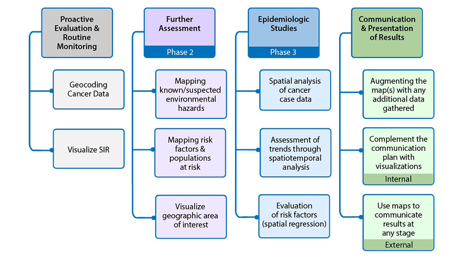
Figure 1: GIS activities throughout the examination of unusual patterns of cancer and environmental concerns
Figure 1 shows geospatial activities suggested for different stages of the examination of unusual patterns of cancer and environmental concerns. Four stages are presented. These stages are proactive evaluation and routine monitoring, further assessment, epidemiologic studies, and communication and presentation of results.
Proactive evaluation and routine monitoring includes:
- Geocoding cancer data
- Visualize SIR
Further Assessment which is associated with Phase 2 includes:
- Mapping known/suspected environmental hazards
- Mapping risk factors and populations at risk
- Visualize geographic area of interest
Epidemiologic studies which are associated with Phase 3 includes:
- Spatial analysis of cancer case data
- Assessment of trends through spatiotemporal analysis
- Evaluation of risk factors (spatial regression)
Communication and presentation of results includes:
- Augmenting the map(s) with any additional data gathered
- Complement the communication plan with visualizations (internal)
- Use maps to communicate results at any stage (external)
Visualization, or mapping, can be used as an important communication tool to both internal and external stakeholders. As part of the routine evaluation of cancer data, maps can be shared with partners in programs such as comprehensive cancer control and environmental health for decision making. Additionally, maps can convey important information about the distribution of cases and potential environmental risk factors when engaging with the community.
Often, a first step in visualization and spatial analysis involves translating addresses collected as text in cancer registry data into coordinates that can be mapped. This process is known as geocoding, and the quality of the result is crucial as it is the basis for visualizations and analyses. Resources are available that provide detailed descriptions of this process123, and tools are available at no cost for health departments from the National Cancer Institute and the North American Association of Central Cancer Registries (NAACCR) Geocoder.
Cancer registries and state health agencies typically have criteria related to release of data for small geographic areas. Because of confidentiality and privacy concerns, some data cannot be released to the public, unless these concerns are addressed. For example, a map of a small geographic area that identifies the residences of cancer patients as points should not be made public4. Similarly, many health agencies are prohibited from publicly releasing a table for a small geographic area with a small population, since each table cell might have only a few cases and could be used to identify individuals.
Once data are geocoded, they can be mapped along with other geographic data, such as suspected environmental risk factors, for crude assessments of their proximity to the cases. Different spatial (e.g., census block, census tract, ZIP Code tabulation area, municipality, or county) or temporal scales (e.g., week, month, year, or several years) can be mapped to look for possible patterns. This practice is more useful when longer periods of time are under study, as well as when there are larger numbers of cases (e.g., >10 cases). Mapping and analyzing the data over space and time can help reveal whether changes in incidence or mortality statistics are observed and may suggest risk factors that warrant further consideration.
Varying the geographic scale or the geographic unit of aggregation can produce different patterns and results. This is known as the modifiable areal unit problem56, which has also been identified relative to temporal aggregations7. Multiple methods have been proposed to account for these issues8910; a common solution is to use differing scales. In doing so, variations in results can be identified if they exist. Further discussion of GIS visualization techniques and methods for the analysis of cancer data are available in the published literature31112.
The following section provides basic information on the principles of clustering methods and statistical considerations when working with spatially structured data. The National Cancer Institute (NCI) provides a variety of methods and tools for analysis of cancer statistics. Some of the tools are more statistical in nature, such as tools to calculate incidence and death rates and trends (available in SEER*Stat), while other visualization and analysis tools are geospatially focused. Access tools and information for further exploration. In addition to these freely available tools, the sections below detail other spatial and statistical methods and software that can be used for these analyses.
Spatial and temporal clusters
Spatial and temporal clusters can be detected by a variety of techniques that evaluate whether similar features, values, or observations are "close" or in close proximity to one another. These techniques can be divided into global, local, and focused methods. A table with methods and associated applications for those categories is available in the Supplemental Information for Appendix B. The table is not meant to be a comprehensive review of applications but rather to provide initial guidance.
Global clustering statistics can be used to determine if there are patterns of clustering anywhere in the study area. Once clustering is deemed likely from global statistics, local clustering methods, including scan statistics, can help to identify clusters within the area of interest. It is worth noting that it is possible to detect statistically significant global clustering without evidence of local clustering and vice versa13. In cases where there is a known point-source, focused tests can be considered. Regression analysis can then be used to understand the association between potential environmental risk factors and cases or to adjust for confounding factors such as latency in cases, mobility, and demographic variables (such as age and race). These methods are further described below, along with example use cases and locations of available software for analysis.
Global clustering methods
Global clustering statistics detect patterns of spatial clustering that occur anywhere in a study area. They do not identify where clusters occur, nor do they identify differences in spatial patterns within the area. One measure of global clustering is spatial autocorrelation, which is the degree of similarity of nearby features. Positive spatial autocorrelation means that features nearby one another have similar values, while negative autocorrelation signifies nearby features that have dissimilar values.
Commonly used methods for testing global clustering are Geary's C14, Moran's I15, and the Oden's Ipop16, which adjusts Moran's I for differences in population. Global clustering can also be assessed using the K-function (Ripley's) when point-level data are available417. GeoDa† and R† packages are publicly available, and several global statistics are available within other proprietary software packages, such as ClusterSeer® † (BioMedware, Ann Arbor, MI), (see Supplemental Information for Appendix B for more information).
Local clustering methods
Local clustering statistics, such as local indicators of spatial autocorrelation (LISA)18, identify the locations of clusters or spatial outliers. Some global clustering statistics have local clustering statistic counterparts such as global and local Moran's I statistics and the Besag-Newell R19. Another statistic, Getis-Ord Gi*, identifies hot and cold spots based on where features with high (hot) or low (cold) values are in close proximity to one another. The Getis-Ord Gi* provides estimates of statistical significance while identifying the locations of hot and cold spots that are not confined to a specific shape.
Local versions of Moran's I and Geary's C are available for free within R† packages such as usdm and spdep20. Other programs also have Moran's I statistics and the Getis-Ord Gi* statistic, such as ArcGIS™ † tools (Esri, Redlands, CA), ClusterSEER†, and GeoDa†21.
Spatial scan statistics can be used to scan a study region using a series of moving windows with increasing radii to identify areas where the observed cases included inside the window are greater than expected. This method can be expanded to incorporate time as an added dimension, allowing a scan for spatiotemporal clusters. To properly interpret the results of the spatial scan statistic, it is extremely important to identify the appropriate radius for the spatial scan window to avoid clusters that are too large or too small. Normally, the upper limit of the circle should not include more than 50 percent of the dataset or the study area422. Additional parameter selection, such as time range and spatial scale within spatial scan statistics, can impact results.
One of the most popular scan statistics is Kulldorff's scan statistic for spatial, temporal, and space-time analysis2324, freely available within SaTScan™ †software25. The SaTScan™ † software includes analyses for different data types including case counts24, rates26, case/control data24, and even survival data27. However, spatial and temporal clusters can appear in irregular shapes, which prompted Tango and Takahashi28 to develop a flexible space-time scan statistic, implemented in the FleXScan† software. The flexscan methodology is also available as an R† package, rflexscan. This package implements both Kulldorff's and Tango & Takahashi's scan statistics.
An alternative scan statistic is that proposed by Besag-Newell29, which is useful for regional data with small population sizes. It is available in the free software ClusterSeer® † This test gives results for both global and local clustering.
Focused clustering tests
A growing interest in recent years has been in the detection of clusters around a specific point-source, such as a single identifiable source of air, water, thermal, noise, or light pollution29. These focused tests are usually designed to identify a particular spatial pattern of clustering around the point-source or specific geographic location. The location of the point-source of interest needs to be identified prior to the assessment, recognizing that different factors (meteorological, topographical, and others) can influence the spatial pattern of potential exposures from the point-source30. The size, shape, and scale of the analysis can also influence the results. For example, below are five focused cluster shapes and corresponding fitted models that can be considered30:
- Distance Decline (DD): A model where risk declines symmetrically in all directions with distance from the point-source
- Peaked Distance Decline (PDD): A model where risk peaks closest to the point-source and then declines with distance
- Direction (D): A model characterizing increased risk in a specific angle/direction from the point-source
- Distance Decline combined with Directional effect (DDIR)
- Peaked Distance Decline combined with Directional effect (PDDIR)
Widely known focused cluster tests prove to have higher relative power for different models:
- Lawson-Waller Score Test: This test provides robust results across different models. This score test is powerful against small deviations from the null in the direction of a specific alternative.3132
- Bithell's Linear Risk Score (LRS) Test: This is a distance version used for DD, PDD; direction version used for D, DDIR, and PDDIR.33
- Cuzick and Edwards' Test: This test performs well for large sample sizes (N>500) and also often used for PDD, DDIR, and PDDIR.34
- Stone's Maximum Likelihood Test: This is used for DD.35
- Tango's Focused Test: This is used for DD.36
- Besag and Newell's Test: This is used for PDD.29
Regression analyses
Regression methods provide analyses and a set of tools that are complementary to cluster detection analysis. Regression analyses are commonly used in public health for two main reasons: 1) to predict an outcome, and 2) to understand the association between at least two variables37. For example, after identifying spatial clusters of cancer cases, it may be useful to understand the relationship between potential environmental exposures and the cancer of interest while controlling for demographic and behavioral factors associated with increased risk3839. Alternatively, it may be of interest to predict the risk of a specific cancer across a wide geographic region if there are data on known environmental exposures39.
Special considerations must be made when applying regression techniques to spatially structured data. Spatially structured data violate a key assumption of independence among observations due to inherent autocorrelation, where a given value is to some degree predicted by the values of its neighbors44041. General steps to overcome issues of spatial autocorrelation in regression, drawing primarily from Waller & Gotway4and Fotheringam & Rogerson42, can be found in the Supplemental Information for Appendix B.
Comparison of methods
The choice of a statistical cluster detection method should take into consideration the strengths and weaknesses of the methods. Several criteria can be considered, such as the type of data (e.g., point-level data or areal data), the ease of use and availability of data or software, the transparency of the methods employed in a particular software, statistical power of the method to detect the cluster of interest, and the desired output35. Multiple comparisons of methods and reviews of techniques have been published over the years1435434445464748495051, and additional details and discussion can be found in the Supplemental Information for Appendix B.
Summary
Cluster detection and other advanced spatial analysis methods are available via proprietary and free applications. Such analysis often requires specialized knowledge about the data, appropriate use of the methods, and careful interpretation of the results. Specifically, the choice of which models to use depends on the type of data, the underlying assumptions based on the distribution of the data, and geospatial considerations such as the size of the study area, spatial scale of the data, aggregation, and masking. For example, results of analysis may greatly differ when implemented at the county or the census tract level, and different models should be implemented if both case and area-level risk factors are evaluated. Specific methods may also require additional considerations such as the type and size of the spatial scan window.
The results of the GIS and spatiotemporal analysis can be used internally for decision making, can inform actions, and can be used to communicate with the public. Therefore, collaborations with GIS professionals and spatial statisticians equipped with specialized skills can help to ensure proper methods are employed and interpretations of results are appropriate. If these experts are not available within the health agency, consultation and technical assistance from CDC/ATSDR's Geospatial Research Analysis and Services Program (GRASP) can be requested by emailing CCGuidelines@cdc.gov.
† Software noted are examples of packages that are available freely or for purchase and do not represent an endorsement of any specific product by the Centers for Disease Control and Prevention or the Agency for Toxic Substances and Disease Registry.
Additional Contributing Authors:
Liora Sahar, Marissa Grossman, Brian Lewis
ATSDR; Geospatial Research, Analysis, and Services Program
- Goldberg DW, Swift JN, Wilson JP. Geocoding Best Practices: Reference Data, Input Data and Feature Matching.
- CDC. Geography and Locational Referencing Subgroup of the Standards and Network Development Workgroup of the National Environmental Public Health Tracking Program. Environmental Public Health Tracking Version 1.0 (A resource for EPHT managers and a tool for their technical staff). 2005.
- Sahar L, Foster SL, Sherman RL, Henry KA, Goldberg DW, Stinchcomb DG, et al. GIScience and cancer: State of the art and trends for cancer surveillance and epidemiology. Vol. 125, Cancer. John Wiley and Sons Inc.; 2019. p. 2544–60.
- Waller LA, Gotway CA. Applied spatial statistics for public health data. New York: John Wiley and Sons; 2004.
- Gehlke CE, Biehl K. Certain Effects of Grouping upon the Size of the Correlation Coefficient in Census Tract Material. J Am Stat Assoc. 1934 Mar;29(185A):169–70.
- Openshaw S, Taylor PJ. A million or so correlation coefficients: Three experiments on the modifiable areal unit problem. Stat Appl Spat Sci. 1979;127–44.
- Cheng T, Adepeju M. Modifiable Temporal Unit Problem (MTUP) and Its Effect on Space-Time Cluster Detection. PLoS One [Internet]. 2014;9(6):1–10. Available from: www.plosone.org
- Wong DW. Modifiable Areal Unit Problem. Int Encycl Hum Geogr. 2009;
- Su MD, Lin M, Wen T. Spatial Mapping and Environmental Risk Identification. 2011.
- Yoo E-H. GIS Methods and Techniques. Compr Geogr Inf Syst. 2018;
- Waller LA, Gotway CA. Applied Spatial Statistics for Public Health Data. Hoboken, NJ: John Wiley & Sons, Inc.; 2004.
- Cromley EK, McLafferty SL. GIS and Public Health. 2nd ed. New York, NY: The Guilford Press; 2012.
- Huang L, Pickle LW, Das B. Evaluating spatial methods for investigating global clustering and cluster detection of cancer cases. Stat Med. 2008 Nov 1;27(25):5111–42.
- Geary RC. The contiguity ratio and statistical mapping. Inc Stat [Internet]. 1954;5(3):115–46. Available from: https://about.jstor.org/terms
- Moran PAP. Notes on continuous stochastic phenomena. Biometrika [Internet]. 1950;37(1/2):17–23. Available from: https://www.jstor.org/stable/2332142
- Oden N. Adjusting Moran's I for population density. Stat Med. 1995;14(1):17–26.
- Ripley BD. Spatial Statistics. New York, NY: John Wiley and Sons; 1981.
- Anselin L. Local indicators of spatial association—LISA. Geogr Anal. 1995;27(2):93–115.
- Costa MA, Assunção RM. A fair comparison between the spatial scan and the Besag-Newell Disease clustering tests. Environ Ecol Stat. 2005;12(3):301–19.
- Naimi B, Hamm NAS, Groen TA, Skidmore AK, Toxopeus AG. Where is positional uncertainty a problem for species distribution modelling? Ecography (Cop). 2014;37(2):191–203.
- Bivand RS, Wong DWS. Comparing implementations of global and local indicators of spatial association. Test [Internet]. 2018;27(3):716–48. Available from: https://doi.org/10.1007/s11749-018-0599-x
- Kulldorff M, Nagarwalla N. Spatial Disease Clusters: Detection and Inference. Vol. 14, STATISTICS IN MEDICINE. 1995.
- Kulldorff M. A spatial scan statistic. Commun Stat methods. 1997;26(6):1481–96.
- Kulldorff M, Heffernan R, Jacobs J, Martins A, Mostashari F. A Space–Time Permutation Scan Statistic for Disease Outbreak Detection. PLoS Med. 2005;2:e59.
- Kulldorff M. Information management services, Inc. SaTScanTM v9. 2009;4.
- Huang L, Tiwari RC, Zou Z, Kulldorff M, Feuer EJ. Weighted Normal Spatial Scan Statistic for Heterogeneous Population Data. J Am Stat Assoc [Internet]. 2009;104(487):886–98. Available from: https://doi.org/10.1198/jasa.2009.ap07613
- Huang L, Kulldorff M, Gregorio D. A spatial scan statistic for survival data. Biometrics. 2007;63(1):109–18.
- Tango T, Takahashi K. A flexibly shaped spatial scan statistic for detecting clusters. Int J Health Geogr. 2005;4(1):1–15
- Besag J, Newell J. The detection of clusters in rare diseases. J R Stat Soc Ser A (Statistics Soc. 1991;154(1):143–55.
- Puett RC, Lawson AB, Clark AB, Aldrich TE, Porter DE, Feigley CE, et al. Scale and shape issues in focused cluster power for count data. Int J Health Geogr. 2005;4(1):1–16.
- Lawson AB. Statistical methods in spatial epidemiology. Wiley; 2006.
- Waller LA, Turnbull BW, Clark LC, Nasca P. Chronic disease surveillance and testing of clustering of disease and exposure: Application to leukemia incidence and TCE-contaminated dumpsites in upstate New York. Environmetrics. 1992;3(3):281–300.
- Bithell JF. The choice of test for detecting raised disease risk near a point source. Stat Med. 1995;14(21–22):2309–22.
- Cuzick J, Edwards R. Methods for investigating localized clustering of disease. Clustering methods based on k nearest neighbour distributions. IARC Sci Publ. 1996;(135):53–67.
- Stone RA. Investigations of excess environmental risks around putative sources: statistical problems and a proposed test. Stat Med. 1988;7(6):649–60.
- Tango T. A class of tests for detecting 'general'and 'focused'clustering of rare diseases. Stat Med. 1995;14(21-22):2323–34.
- Kleinbaum DG, Kupper LL, Nizam A, Rosenberg ES. Applied regression analysis and other multivariable methods. 5th ed. Boston, MA, USA: Cengage Learning; 2013. 1074 p.
- Cardoso D, Painho M, Roquette R. A geographically weighted regression approach to investigate air pollution effect on lung cancer: A case study in Portugal. Geospat Heal. 2019/05/18. 2019;14(1).
- Elliott P, Wartenberg D. Spatial epidemiology: current approaches and future challenges. Env Heal Perspect [Internet]. 2004/06/17. 2004;112(9):998–1006. Available from: https://www.ncbi.nlm.nih.gov/pubmed/15198920
- Fotheringham AS. "The Problem of Spatial Autocorrelation" and Local Spatial Statistics. Geogr Anal [Internet]. 2009;41(4):398–403. Available from: https://onlinelibrary.wiley.com/doi/abs/10.1111/j.1538-4632.2009.00767.x
- Legendre P. Spatial Autocorrelation: Trouble or New Paradigm? Ecology [Internet]. 1993;74(6):1659–73. Available from: https://esajournals.onlinelibrary.wiley.com/doi/abs/10.2307/1939924
- Fotheringham AS, Rogerson PA. The SAGE handbook of spatial analysis [Internet]. Thousand Oaks, CA, USA: Sage; 2009. p. 528. Available from: https://methods.sagepub.com/Book/the-sage-handbook-of-spatial-analysis
- Goujon S, Kyrimi E, Faure L, Guissou S, Hémon D, Lacour B, et al. Spatial and temporal variations of childhood cancers: Literature review and contribution of the French national registry. Cancer Med. 2018;7(10):5299–314.
- Kulldorff M, Huang L, Pickle L, Duczmal L. An elliptic spatial scan statistic. Stat Med. 2006;25(22):3929–43.
- Lin H, Ning B, Li J, Ho SC, Huss A, Vermeulen R, et al. Lung cancer mortality among women in Xuan Wei, China: a comparison of spatial clustering detection methods. Asia Pacific J Public Heal. 2015;27(2):NP392–401.
- Hanson CE, Wieczorek WF. Alcohol mortality: a comparison of spatial clustering methods. Soc Sci Med. 2002;55(5):791–802.
- Kim J, Lee M, Jung I. A comparison of spatial pattern detection methods for major cancer mortality in Korea. Asia Pacific J Public Heal. 2016;28(6):539–53.
- Chen J, Roth RE, Naito AT, Lengerich EJ, MacEachren AM. Geovisual analytics to enhance spatial scan statistic interpretation: an analysis of US cervical cancer mortality. Int J Health Geogr. 2008;7(1):1–18.
- Kulldorff M, Song C, Gregorio D, Samociuk H, DeChello L. Cancer map patterns: are they random or not? Am J Prev Med. 2006;30(2):S37–49.
- Jackson MC, Huang L, Luo J, Hachey M, Feuer E. Comparison of tests for spatial heterogeneity on data with global clustering patterns and outliers. Int J Health Geogr. 2009;8(1):1–14.
- Tango T. Spatial scan statistics can be dangerous. Stat Methods Med Res. 2021;30(1):75–86.